Construct a continuous area cartogram by a rubber sheet distortion algorithm (Dougenik et al. 1985)
Usage
cartogram_cont(
  x,
  weight,
  itermax = 15,
  maxSizeError = 1.0001,
  prepare = "adjust",
  threshold = "auto",
  verbose = FALSE,
  n_cpu = getOption("cartogram_n_cpu", "respect_future_plan"),
  show_progress = getOption("cartogram.show_progress", TRUE)
)

# S3 method for class 'SpatialPolygonsDataFrame'
cartogram_cont(
  x,
  weight,
  itermax = 15,
  maxSizeError = 1.0001,
  prepare = "adjust",
  threshold = "auto",
  verbose = FALSE,
  n_cpu = getOption("cartogram_n_cpu", "respect_future_plan"),
  show_progress = getOption("cartogram.show_progress", TRUE)
)

# S3 method for class 'sf'
cartogram_cont(
  x,
  weight,
  itermax = 15,
  maxSizeError = 1.0001,
  prepare = "adjust",
  threshold = "auto",
  verbose = FALSE,
  n_cpu = getOption("cartogram_n_cpu", "respect_future_plan"),
  show_progress = getOption("cartogram.show_progress", TRUE)
)
Arguments
- x
a polygon or multiplogyon sf object
- weight
Name of the weighting variable in x
- itermax
Maximum iterations for the cartogram transformation, if maxSizeError ist not reached
- maxSizeError
Stop if meanSizeError is smaller than maxSizeError
- prepare
Weighting values are adjusted to reach convergence much earlier. Possible methods are:
"adjust", adjust values to restrict the mass vector to the quantiles defined by threshold and 1-threshold (default),
"remove", remove features with values lower than quantile at threshold,
"none", don't adjust weighting values
- threshold
"auto" or a threshold value between 0 and 1. With “auto”, the value is 0.05 or, if the proportion of zeros in the weight is greater than 0.05, the value is adjusted accordingly.
- verbose
print meanSizeError on each iteration
- n_cpu
Number of cores to use. Defaults to "respect_future_plan". Available options are:
"respect_future_plan" - By default, the function will run on a single core, unless the user specifies the number of cores using
plan(e.g.future::plan(future::multisession, workers = 4)) before running thecartogram_contfunction."auto" - Use all except available cores (identified with
availableCores) except 1, to keep the system responsive.a
numericvalue - Use the specified number of cores. In this casecartogram_contwill use set the specified number of cores internally withfuture::plan(future::multisession, workers = n_cpu)and revert that back by switching the plan back to whichever plan might have been set before by the user. If only 1 core is set, the function will not requirefutureandfuture.applyand will run on a single core.
- show_progress
A
logicalvalue. If TRUE, show progress bar. Defaults to TRUE.
References
Dougenik, J. A., Chrisman, N. R., & Niemeyer, D. R. (1985). An Algorithm To Construct Continuous Area Cartograms. In The Professional Geographer, 37(1), 75-81.
Examples
# ========= Basic example =========
library(sf)
#> Linking to GEOS 3.12.1, GDAL 3.8.4, PROJ 9.4.0; sf_use_s2() is TRUE
library(cartogram)
nc = st_read(system.file("shape/nc.shp", package="sf"), quiet = TRUE)
# transform to NAD83 / UTM zone 16N
nc_utm <- st_transform(nc, 26916)
# Create cartogram
nc_utm_carto <- cartogram_cont(nc_utm, weight = "BIR74", itermax = 5)
# Plot
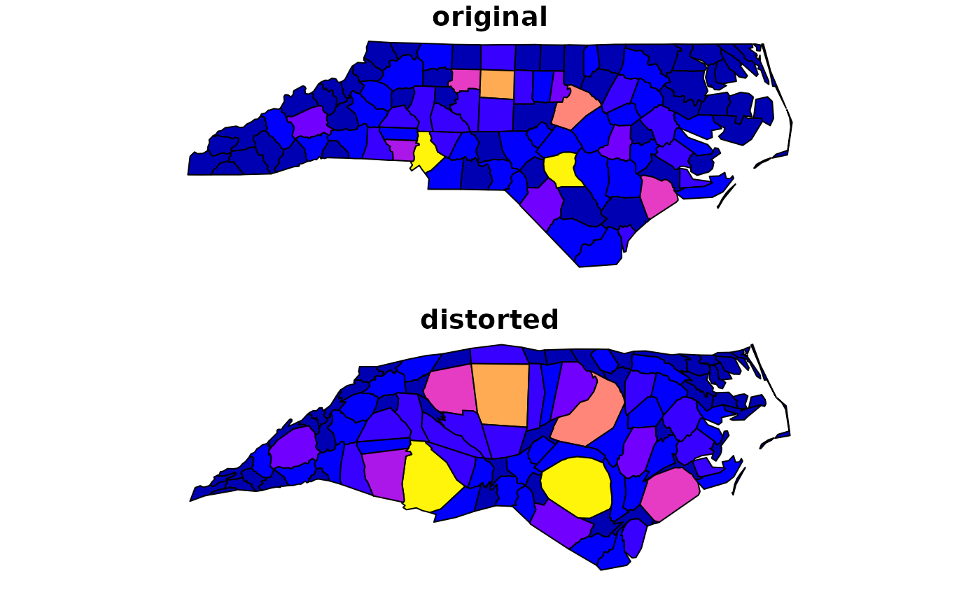
par(mfrow=c(2,1))
plot(nc[,"BIR74"], main="original", key.pos = NULL, reset = FALSE)
plot(nc_utm_carto[,"BIR74"], main="distorted", key.pos = NULL, reset = FALSE)
 # ========= Advanced example 1 =========
# Faster cartogram using multiple CPU cores
# using n_cpu parameter
library(sf)
library(cartogram)
nc = st_read(system.file("shape/nc.shp", package="sf"), quiet = TRUE)
# transform to NAD83 / UTM zone 16N
nc_utm <- st_transform(nc, 26916)
# Create cartogram using 2 CPU cores on local machine
nc_utm_carto <- cartogram_cont(nc_utm, weight = "BIR74", itermax = 5,
n_cpu = 2)
# Plot
par(mfrow=c(2,1))
plot(nc[,"BIR74"], main="original", key.pos = NULL, reset = FALSE)
plot(nc_utm_carto[,"BIR74"], main="distorted", key.pos = NULL, reset = FALSE)
# ========= Advanced example 2 =========
# Faster cartogram using multiple CPU cores
# using future package plan
# \donttest{
library(sf)
library(cartogram)
library(future)
nc = st_read(system.file("shape/nc.shp", package="sf"), quiet = TRUE)
# transform to NAD83 / UTM zone 16N
nc_utm <- st_transform(nc, 26916)
# Set the future plan with 2 CPU local cores
# You can of course use any other plans, not just multisession
future::plan(future::multisession, workers = 2)
# Create cartogram with multiple CPU cores
# The cartogram_cont() will respect the plan set above
nc_utm_carto <- cartogram_cont(nc_utm, weight = "BIR74", itermax = 5)
# Shutdown the R processes that were created by the future plan
future::plan(future::sequential)
# Plot
par(mfrow=c(2,1))
plot(nc[,"BIR74"], main="original", key.pos = NULL, reset = FALSE)
plot(nc_utm_carto[,"BIR74"], main="distorted", key.pos = NULL, reset = FALSE)
# }
# ========= Advanced example 1 =========
# Faster cartogram using multiple CPU cores
# using n_cpu parameter
library(sf)
library(cartogram)
nc = st_read(system.file("shape/nc.shp", package="sf"), quiet = TRUE)
# transform to NAD83 / UTM zone 16N
nc_utm <- st_transform(nc, 26916)
# Create cartogram using 2 CPU cores on local machine
nc_utm_carto <- cartogram_cont(nc_utm, weight = "BIR74", itermax = 5,
n_cpu = 2)
# Plot
par(mfrow=c(2,1))
plot(nc[,"BIR74"], main="original", key.pos = NULL, reset = FALSE)
plot(nc_utm_carto[,"BIR74"], main="distorted", key.pos = NULL, reset = FALSE)
# ========= Advanced example 2 =========
# Faster cartogram using multiple CPU cores
# using future package plan
# \donttest{
library(sf)
library(cartogram)
library(future)
nc = st_read(system.file("shape/nc.shp", package="sf"), quiet = TRUE)
# transform to NAD83 / UTM zone 16N
nc_utm <- st_transform(nc, 26916)
# Set the future plan with 2 CPU local cores
# You can of course use any other plans, not just multisession
future::plan(future::multisession, workers = 2)
# Create cartogram with multiple CPU cores
# The cartogram_cont() will respect the plan set above
nc_utm_carto <- cartogram_cont(nc_utm, weight = "BIR74", itermax = 5)
# Shutdown the R processes that were created by the future plan
future::plan(future::sequential)
# Plot
par(mfrow=c(2,1))
plot(nc[,"BIR74"], main="original", key.pos = NULL, reset = FALSE)
plot(nc_utm_carto[,"BIR74"], main="distorted", key.pos = NULL, reset = FALSE)
# }